Introduction
PSNToolsGUI is a easy-to-use software with a graphical user interface for calculating and analyzing Protein Structure Networks (PSN) from both single structures and molecular dynamics trajectories for high throughput investigation of allosterism in biological systems. PSNToolsGUI employs a mixed strategy integrating PSN and the correlations of the atomic fluctuations to investigate the structural communication in proteins and nucleic acids.
The PSN analysis proved as valuable tools in a number of studies and PSNToolsGUI provides the user with a easy to use and an immediate feedback through easily accessible data files and graphical visualizations of the output. Automation, high speed and the broad range of available network analyses make this software suitable for high throughput investigation of the communication pathways in large sets of biomolecular systems in different functional states.
Despite the large number of provided options and alternative algorithms PSNToolsGUI will automatically set benchmark proved values tested against experimental data. For more details about published papers and the theory behind PSN analysis, please visit WebPSN webserver.
PSNToolsGUI is user friendly, lightweight and has a consistent graphical user interface for a gentle and gradual learning curve. Finally, PSNToolsGUI has a periodically updated internal database of more than 30,000 pre-calculated network parameters for ions and other molecules present in all PDB structures.
Please note that this guide is about PSNToolsGUI only, please refer to the PSNTools user guide and to WebPSN webserver for more details.
Installation and Requirements
PSNToolsGUI is free and open to all users and is distributed as a binary executable (recommended) and as source code which can be compiled on other platforms. Both the binary and the source code can be downloaded at the website of WebPSN server.
The binary executable has been tested to properly work out of the box using a fresh install of the latest two releases of the following, widely used, Linux distributions: Ubuntu, Fedora and Manjaro.
Compilation can be (very) long due to the large internal database of network parameters and requires a modern C++ compiler and toolchain and the following development libraries: Boost, Cereal, ZLib, Armadillo and BLAS/LAPACK libraries.
PSNToolsGUI uses the command line version of PSNTools and, for some calculation stages, Wordom, another software provided by the same research group. A statically compiled binary executable for Wordom is provided as well. To use PSNToolsGUI, PSNTools and Wordom you can download (or compile) the executable files and move them to an appropriate location in your filesystem. The only additional requirement to run PSNToolsGUI is a complete installation of the Python 2.7 programming language, which is already present by default in almost all linux distributions.
Finally, this is a list of additional recommended software that, while not strictly necessary, are however highly recommended: PyMol, VMD, Gnuplot, Graphviz.
Please, refer to your operating system manual and to the website of each software for more details about the installation process:
How to Cite
Thank you for using PSNToolsGUI, we really appreciate it.
Please, remember to cite at least one of the following papers in all published works which utilize this software:
NEW_PAPER_CITATION_HERE
Angelo Felline, Michele Seeber and Francesca Fanelli
webPSN v2.0: a webserver to infer fingerprints of structural communication in biomacromolecules
Nucleic Acids Res, Web Server Issue, 19 May 2020
https://doi.org/10.1093/nar/gkaa397
Contacting Us
If you have any questions or if you encounter any problems with this sofware please do not hesitate to contact us at the following email addresses:
Copyright and Disclaimer Notices
PSNToolsGUI is copyright 2017-2020 the University of Modena and Reggio Emilia (Italy).
PSNToolsGUI is free software; you can redistribute it and/or modify it under the terms of the GNU General Public License as published by the Free Software Foundation; either version 3 of the License, or (at your option) any later version.
PSNToolsGUI is distributed in the hope that it will be useful, but WITHOUT ANY WARRANTY; without even the implied warranty of MERCHANTABILITY or FITNESS FOR A PARTICULAR PURPOSE. See the GNU General Public License for more details.
You should have received a copy of the GNU General Public License along with Wordom. If not, see http://www.gnu.org/licenses
First Run and Configuration
This is the main window of PSNToolsGUI

All PSNToolsGUI functions can be easily accessed from the main menu which will be detailed later in this guide. At the first run after installation, you will be asked to complete your configuration.

All your configurations will be saved in a text file called .psntools-gui.rc automatically created in your home directory. You can either, edit manually this file or use the Configuration menu.

This configuration stage is used to set the external software called by PSNToolsGUI to open its output files. For each software you need to set the full path to the executable file or just the executable name if it is in path. You can set the following software:
-
psntools: psntools command line executable
-
wordom: wordom executable
-
Text Editor: your favorite text editor (e.g. nedit)
-
Spreadsheet: your favorite spreadsheet software (e.g. libreoffice --calc)
-
Image Viewer: your favorite image viewer (e.g. eog)
-
PDF Viewer: your favorite image viewer (e.g. evince)
-
PyMol: pymol executable (e.g. just pymol should be fine)
-
VMD: vmd executable (e.g. just vmd should be fine)
If you click on "Config File", the configuration file will be opened for manual editing.
Calculate Menu
In order to perform a network analysis you need to calculate a network first, using the Calculate Menu.

This menu can be used to calculate a network from a single pdb file or from a pdb file and a trajectory file in DCD or XTC format. Additionally, you can also calculate a Consensus network combining together two or more, previously calculated, networks.
Network Calculation
To calculate a Protein Structure Network from a single PDB file or a Gromacs (xtc) or CHARMM (dcd) trajectory file click on Calculate → PSN to calculate a new network. For detailed information on the theory behind this step, read the relevant section in the Appendices chapter.

the following new window will be opened:
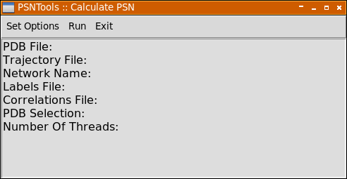
Use Set Options menu to setup your calculation. Each menu entry is marked as Required or Optional, and all optional settings will be automatically adjusted for you depending on the situation.

| Item | Description |
|---|---|
PDB File |
Will open a file selection dialog to select a pdb file |
Trajectory File |
Will open a file selection dialog to select a dcd or a xtc file |
Network name |
Will open a input dialog that can be used to insert a network name, if not used the pdb file name will be used |
Labels File |
Will open a file selection dialog to select a labels file |
Labels File |
Will open a file selection dialog to select a labels file |
Corr. File |
Will open a file selection dialog to select a correlations file |
Selection |
Will open a input dialog that can be used to enter a selection string |
Number Of Threads |
Will open a input dialog that can be used to enter the number of threads |
Please, refer to the PSNTools user guide for more details about the meanings of these options.
To calculate your network click on Run → Calculate PSN. Finally, click on Exit to close this window.
Consensus Calculation
Computation of consensus networks allows inferring common structural communication features in homologous systems sharing the same functionality or even only the fold. A consensus network is calculated by averaging the trajectory frequencies and interactions strengths of all hubs and links among the networks used to build the consensus. Once produced, the .psn file of a consensus network can be used as a normal network and can be analyzed using the methods present in Analyses menu.
Click on Calculate → Consensus to calculate a new consensus network.

As for the network calculation procedure you can setup the consensus calculation using the Set Options menu.

The only required option you have to provide is the list of psn files you want to use to calculate your consensus network. You have to select two or more psn files using Set Options → PSN Files menu (You have to hold your ctrl down while selecting multiple files).
When the calculation is finished you can close this window using Exit menu.
Analyses Menu
This menu is used to run the vast majority of network analyses available in PSNToolsGUI.
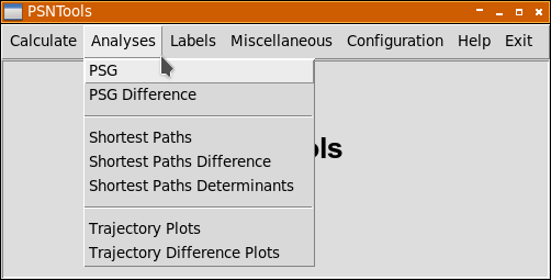
Each analysis has its own window and it is possible to run multiple analyses in parallel.
Network Representation
After the PSN calculation stage, you can use the produced .psn file to generate a network representation called Protein Structure Graph (PSG) clicking on Analyses → PSG Menu. Please remember that all optional values listed below will be automatically set for you to a reasonable default value.

The following options are available in the Set Options menu:
| Option | Description |
|---|---|
PSN File |
Used to select a .psn file calculated with the Calculate → PSN or Calculate → Consensus. Required. |
Network Name |
If used, all resulting output files will be named according to the value passed to this option, otherwise the internal network name will be used (defualt). Optional. |
Labels File |
Select a labels file, if passed the nodes in the resulting outputs will be labeled according to this file. Please note that in order to properly work you need a unlabeled .psn file. Optional. |
External Values File |
This option is used to select an external numerical values (i.e. sequence conservation data, experimental values, etc). These values will be reported in the output files alongside network values. These external numerical values file are formatted in the vein of labels files. See External Values File section for more details. Optional. |
Include Glycines |
If true (default) glycines will be included in all calculations and representations. Optional. |
Minimum Frequency |
This option accepts a numerical value > 0 and ≤ 100. Links and Hubs (read the relevant section in the Appendices chapter for more details) will be considered only if their frequency (i.e. % of trajectory frames) is ≥ than this value. The default is 50. Optional. |
Clust. Merging Algo. |
This option is used to set the clusters merging criterion (read the relevant section in the Appendices chapter for more details) and accepts one of the following values: no, imin, imin2, freq. Optional. |
When all desired options has been set, you can calculate the PSG using Run → Calculate PSG menu. When the calculation is finished, the Outputs menu will be automatically activated:
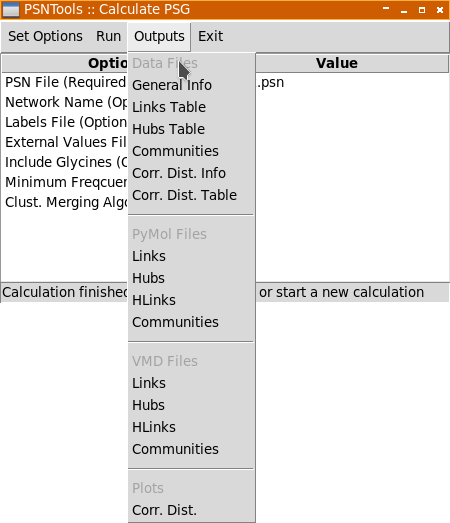
Output files are grouped as follow:
-
Data Files: text files opened with selected text editor or spreadsheet software.
-
PyMol/VMD Files: 3D scripts files passed to PyMol and VMD, respectively.
-
Plots: plots and images that will opened by selected image viewer.
Please, see First Run and Configuration section for more details.
The following output files will be available:
| Output | Description |
|---|---|
General Info |
This file contains a summary of calculated PSG:
|
Links Table |
This file contains a detailed table listing all the links in the calculated network with the following information:
|
Hubs Table |
This file contains a detailed table inherent the hubs in the calculated network with the following information:
|
Communities |
This file contains a detailed summary of all node communities in calculated network. For each community, listed from the larger to the smaller, the following information are provided:
For each community the list of all its links is also provided with the following additional information:
|
Corr. Dist. Info |
This file contains a table with a number of statistics relative to the correlations of the atomic fluctuations.
|
Corr. Dist. Table |
This file contains the data used to produce the plot Corr. Dist. |
| Output | Description |
|---|---|
Links |
These scripts display all the links in the calculated PSG. Please, refer to section for details about used colors. |
Hubs |
These scripts display all the hubs in the calculated network. Please, refer to section for details about used colors. |
HLinks |
These scripts display all the links mediated by at least one hub in the calculated network. Please, refer to section for details about used colors. |
Communities |
These scripts display communities of nodes identified in the calculated network. Nodes are represented as spheres centered on the Calpha (for standard aminoacids) or geometric center for all other molecule, while links are represented as sticks that connect two nodes. Each community is represented with a unique color and nodes and links belonging to the same community share the same colors. The colors of the first nine most populous communities can be seen in the appropriate section. |
| Output | Description |
|---|---|
Corr. Dist. |
This plot represent the distribution of the correlations of the atomic fluctuations versus the % of node pairs. |
Finally, you can close this window using Exit menu.
Network Difference
Network difference is used to highlight the differences between two PSGs in terms of their links, hubs and links mediated by at least one hub. This analysis is particularly useful to identify commonalties and differences in the structural communication of two functionally different states of the same system. Please remember that you need to pass one or two labels files if the two networks have a different primary sequence or even they have the same sequence but different chains and/or segments in the passed pdb files. Please see Labels File section for more details. Please remember that all optional values listed below will be automatically set for you to a reasonable default value.
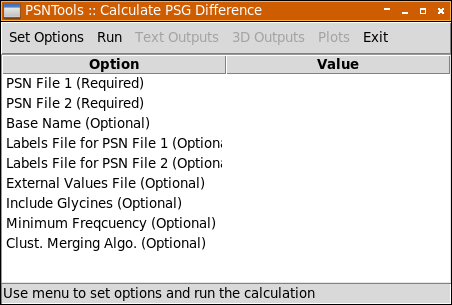
The following options are available in the Set Options menu:
| Option | Description |
|---|---|
PSN File 1 and PSN File 2 |
Use these options to select the two .psn files to be analyzed. Required. |
Base Name |
If used, all resulting output files will be named according to the value passed to this option, otherwise "psndiff_" will be used (defualt). Optional. |
Labels File 1 and Labels File 2 |
Use these options to select the labels files. If the two networks have a different primary sequence or even if they have the same sequence but their pdb files have different chains and/or segments you need to use this option. -labfile1 is used to select the labels file to be applied to the .psn file passed to -psn1 option, while -labfile2 is used for the .psn file passed to -psn2. Additionally, you can use -labfile option to apply the same labels to both network. Please note that in order to properly work you need a unlabeled .psn file (i.e. you need to calculate your .psn file without -labfile option). See -calc command and Labels File section for more details. Optional. |
External Values File |
This option is used to select an external numerical values (i.e. sequence conservation data, experimental values, etc). These values will be reported in the output files alongside network values. These external numerical values file are formatted in the vein of labels files. See External Values File section for more details. Optional. |
Include Glycines |
If true (default) glycines will be included in all calculations and representations. Optional. |
Minimum Frequency |
This option accepts a numerical value > 0 and ≤ 100. Links and Hubs (read the relevant section in the Appendices chapter for more details) will be considered only if their frequency (i.e. % of trajectory frames) is ≥ than this value. The default is 50. Optional. |
Clust. Merging Algo. |
This option is used to set the clusters merging criterion (read the relevant section in the Appendices chapter for more details) and accepts one of the following values: no, imin, imin2, freq. Optional. |
When all desired options has been set, you can calculate the PSG Difference using Run → Calculate PSG Difference menu. When the calculation is finished, the following outputs menus will be automatically activated:
Output files are grouped as follow:
-
Text Files: text output files that will be opened with selected text editor or spreadsheet software.
-
3D Files: 3D scripts files passed to PyMol and VMD, respectively.
-
Plots: plots and images that will opened by selected image viewer.
Please, see First Run and Configuration section for more details.
| Output | Description |
|---|---|
General Info |
This file contains a summary of calculated network difference:
|
Links Table |
This table summarize the differences about shared and common hubs between the two networks.
|
Hubs Table |
This table summarize the differences about shared and common hubs between the two networks.
|
Perturbed Links Table |
These tables summarize the perturbation of each hub/link in both networks using the equation defined in the description of the -pert option. These tables share the very same structure and only the first one is described here.
|
Corr. Dist. Info |
This file contains a table with a number of statistics relative to the correlations of the atomic fluctuations.
|
Corr. Dist. Table |
This file contains the data used to produce the plot Corr. Dist. |
The outputs accessible in 3D Outputs menu are divided in PyMol and VMD groups and then in Net1 vs Net2 and Net2 vs Net1.
| Output | Description |
|---|---|
Links Diff. |
These 3D scripts compare the different links present in both networks. Links specific of the first, second and those links share by the two networks are represented in orange, purple and green. Nodes linked by these links follow the same color scheme. |
Hubs Diff. |
These 3D scripts compare the different hubs present in both networks. Hubs specific of the first, second and those links share by the two networks are represented in orange, purple and green. Nodes linked by these links follow the same color scheme. |
All/Neg./Pos. Pert. Links |
All these 3D script files show the perturbation of each link in the two analyzed networks. Those files with the _pos_ in their name, show only those links with a perturbation > 0, while those files with _neg_ in their name, show only those links with a perturbation < 0. Finally, those files with _all_ in their name, show both, negative and positive perturbed links. |
All/Neg./Pos. Pert. Hubs |
All these 3D script files can be used to visualize the perturbation of each hub in the two analyzed networks. Those files with the _pos_ in their name, show only those hubs with a perturbation > 0, while those files with _neg_ in their name, show only those hubs with a perturbation < 0. Finally, those files with _all_ in their name, show both, negative and positive perturbed hubs. |
The outputs accessible in Plots menu are:
| Output | Description |
|---|---|
Corr. Dist. |
This plot is a graphical comparison between the two analyzed networks of the distributions of the correlations of the atomic fluctuations versus the % of node pairs. |
Spec. Linked Nodes |
This histogram shows the total number of nodes with at least one link in both networks. |
Shared Linked Nodes |
This histogram shows the number of specific and shared linked nodes |
Spec. Links |
This histogram shows the total number of links in both networks. |
Shared Links |
This histogram shows the number of specific and shared links nodes |
Spec. Hubs |
This histogram shows the total number of hubs in both networks. |
Shared Hubs |
This histogram shows the number of specific and shared hubs nodes |
HLinks |
This histogram shows the total number of links mediated by at least one hub in both networks. |
Finally, use Exit menu to close this window.
Shortest Communication Paths
After the PSN calculation stage, you can use the produced .psn file to calculate the correlated shortest communication path(s) between two or more nodes clicking on Analyses → Shortest Paths. As for the previous commands, remember that all optional values listed below will be automatically set for you to a reasonable default value.

As for the the other analyses provided by PSNToolsGUI you can setup all required and optional settings using Set Options menu.
| Option | Description |
|---|---|
PSN File |
Used to select a .psn file calculated with the Calculate → PSN or Calculate → Consensus. Required. |
Network Name |
If used, all resulting output files will be named according to the value passed to this option, otherwise the internal network name will be used (defualt). Optional. |
Labels File |
Select a labels file, if passed the nodes in the resulting outputs will be labeled according to this file. Please note that in order to properly work you need a unlabeled .psn file. Optional. |
External Values File |
This option is used to select an external numerical values (i.e. sequence conservation data, experimental values, etc). These values will be reported in the output files alongside network values. These external numerical values file are formatted in the vein of labels files. See External Values File section for more details. Optional. |
Include Glycines |
If true (default) glycines will be included in all calculations and representations. Optional. |
Minimum Frequency |
This option accepts a numerical value > 0 and ≤ 100. Links and Hubs (read the relevant section in the Appendices chapter for more details) will be considered only if their frequency (i.e. % of trajectory frames) is ≥ than this value. The default is 50. Optional. |
Minimum Recurrence |
This option accepts a numerical value > 0 and ≤ 100 and is used to set the minimum metapath recurrence. The default is 10 and 20 for networks calculated from a pdb or a trajectory file, respectively. Optional. |
Minimum Correlation |
This option accepts a numerical value > 0 and ≤ 1 and is used to set the minimum correlation of the atomic fluctuations. This option, combined with -corrmode, is used to filter out shortest paths with poor correlation. The default is 0.7 and 0.8 for networks calculated from a pdb or a trajectory file, respectively. Optional. |
Clust. Merging Algo. |
This option is used to set the clusters merging criterion (read the relevant section in the Appendices chapter for more details) and accepts one of the following values: no, imin, imin2, freq. Optional. |
Number Of Threads |
This option set the number of threads used to speedup shortest paths calculation. If you are working on a multi-cores workstation, a large value is advisable. 1 by default. Optional. |
Tail Node(s) |
Select only those shortest paths that start or end to a given node. This option also accepts a list of space separated nodes. See Selection Syntax for more details about accepted syntax. Optional. |
Node Pair(s) |
Calculate the shortest paths between a pair of nodes. Nodes in a pair are separated by a "," character. Multiple pairs can be passed by separating pairs with a space character. See Selection Syntax for more details about accepted syntax. Optional. |
Midway Node(s) |
Select only those shortest paths that pass through a given node. This option also accepts a list of space separated nodes. See Selection Syntax for more details about accepted syntax. Optional. |
When all desired options has been set, you can calculate the PSG Difference using Run → Calculate Shortest Paths menu. When the calculation is finished, Outputs menu will be automatically activated giving access to the following outputs:
| Output | Description |
|---|---|
General Info |
This file summarizes the value of all used options in the performed shortest paths calculation. |
Paths Info |
This file reports a series of statistics about the filtered shortest paths pool.
|
Paths Table |
This file reports a series of information for each path in the shortest path pool.
|
Metapath Table |
These files report a series of information about all the links present in the filtered shortest paths pool. The former file lists only those links which respect the filtering criteria of -mpselemode and -rec options, while the latter lists all links.
|
Metapath Table (rec = 0) |
Similar to the previous output file but Minimum Recurrence option set to 0. |
Corr. Dist. |
This data file reports the distribution of the average correlation between the each node and the first and last nodes in each path present in the shortest path pool. |
Corr. Fract. Dist. |
This data file reports the distribution of the percentage of nodes with a correlation with the first and/or the last node in each path present in the shortest path pool. |
Interaction Strengths Dist. |
This data file reports the distribution of the average interaction strength of the links in each path present in the shortest path pool. |
Hubs Dist. |
This data file reports the distribution of the percentage of hubs in each path present in the shortest path pool. |
Length Dist. |
This data file reports the distribution of the number of nodes in each path present in the shortest path pool. |
| Output | Description |
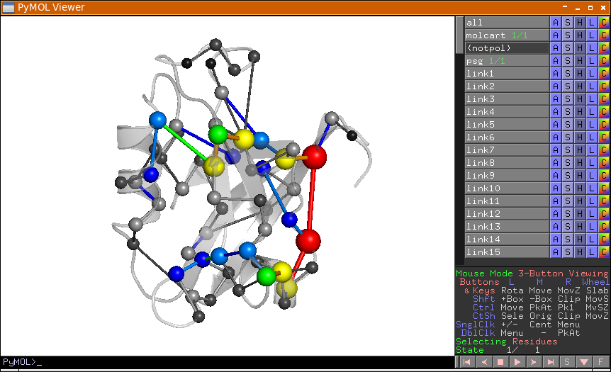
|---|---|
Metapath (PyMol/VMD) |
These 3D scripts represent the coarse communication pathway in the analyzed network using the filtered shortest paths pool. |
| Output | Description |
|---|---|
Metapath 2D |
This image is a 2D representation of the computed metapath. |
Corr. Dist. |
This plot reports the distribution of the average correlation between the each node and the first and last nodes in each path present in the shortest path pool. |
Corr. Fract. Dist. |
This plot reports the distribution of the percentage of nodes with a correlation with the first and/or the last node in each path present in the shortest path pool. |
Interaction Strengths Dist. |
This plot reports the distribution of the average interaction strength of the links in each path present in the shortest path pool. |
Hubs Dist. |
This plot reports the distribution of the percentage of hubs in each path present in the shortest path pool. |
Length Dist. |
This plot reports the distribution of the number of nodes in each path present in the shortest path pool. |
Finally, you can close this window using Exit menu.
Shortest Paths Difference
This analysis is used to perform and compare the results of shortest paths analysis of two networks. Most of the options accepted by this command are the same of those accepted by Shortest Paths analysis and their values can be conveniently applied to both networks.. As always, all non used options will be set to reasonable default values.
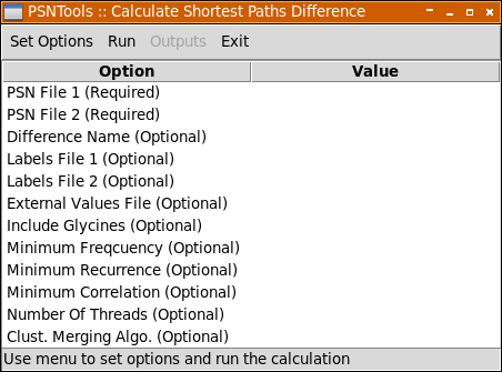
As for the the other analyses provided by PSNToolsGUI you can setup all required and optional settings using Set Options menu.
| Option | Description |
|---|---|
PSN File 1 |
Used to select the .psn files to be analyzed. Required. |
Difference Name |
If used, all resulting output files will be named according to the value passed to this option. Default is pathsdiff. Optional. |
Labels File 1 |
Select the two labels file, if passed the nodes in the resulting outputs will be labeled according to this file. Please note that in order to properly work you need a unlabeled .psn file. Optional. |
External Values File |
This option is used to select an external numerical values (i.e. sequence conservation data, experimental values, etc). These values will be reported in the output files alongside network values. These external numerical values file are formatted in the vein of labels files. See External Values File section for more details. Optional. |
Include Glycines |
If true (default) glycines will be included in all calculations and representations. Optional. |
Minimum Frequency |
This option accepts a numerical value > 0 and ≤ 100. Links and Hubs (read the relevant section in the Appendices chapter for more details) will be considered only if their frequency (i.e. % of trajectory frames) is ≥ than this value. The default is 50. Optional. |
Minimum Recurrence |
This option accepts a numerical value > 0 and ≤ 100 and is used to set the minimum metapath recurrence. The default is 10 and 20 for networks calculated from a pdb or a trajectory file, respectively. Optional. |
Minimum Correlation |
This option accepts a numerical value > 0 and ≤ 1 and is used to set the minimum correlation of the atomic fluctuations. This option, combined with -corrmode, is used to filter out shortest paths with poor correlation. The default is 0.7 and 0.8 for networks calculated from a pdb or a trajectory file, respectively. Optional. |
Clust. Merging Algo. |
This option is used to set the clusters merging criterion (read the relevant section in the Appendices chapter for more details) and accepts one of the following values: no, imin, imin2, freq. Optional. |
Number Of Threads |
This option set the number of threads used to speedup shortest paths calculation. If you are working on a multi-cores workstation, a large value is advisable. 1 by default. Optional. |
Tail Node(s) |
Select only those shortest paths that start or end to a given node. This option also accepts a list of space separated nodes. See Selection Syntax for more details about accepted syntax. Optional. |
Node Pair(s) |
Calculate the shortest paths between a pair of nodes. Nodes in a pair are separated by a "," character. Multiple pairs can be passed by separating pairs with a space character. See Selection Syntax for more details about accepted syntax. Optional. |
Midway Node(s) |
Select only those shortest paths that pass through a given node. This option also accepts a list of space separated nodes. See Selection Syntax for more details about accepted syntax. Optional. |
When all desired options has been set, you can calculate the PSG Difference using Run → Calculate Shortest Paths Difference menu. When the calculation is finished, Outputs menu will be automatically activated giving access to the following outputs:
| Output | Description |
|---|---|
General Info |
This file is a summary of the two calculated metapaths.
|
Metapath Table |
This file has a detailed table of the metapath links of both networks
|
| Output | Description |
|---|---|
Metapath Diff … |
These 3D scripts represent the difference between the two metapaths. |
| Output | Description |
|---|---|
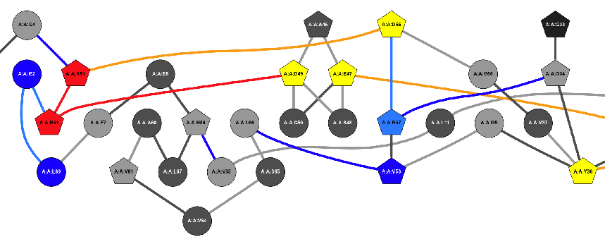
Metapath Diff. 2D … |
These images are 2D representations of the computed metapath difference. |
Num Of Paths Hist. |
This histogram shows the difference in the total number of shortest paths in the two networks. |
Corr. Hist. |
These plots are the average correlation of the filtered shortest paths pool in the two networks, the distributions of the residue average correlations plotted versus the total number of shortest paths and the % of total shortest paths, respectively. |
Corr. Fract. Hist. |
These plots are the average fraction of correlated residues of the filtered shortest paths pool in the two networks and the distributions of the fraction of correlated residues plotted versus the total number of shortest paths and the % of total shortest paths, respectively. |
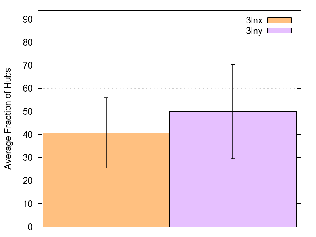
Hubs Fract. Hist. |
These plots are the average correlation of the filtered shortest paths pool in the two networks and the distributions of the hubs % present in each path plotted versus the total number of shortest paths and the % of total shortest paths, respectively. |
Interaction Strengths. Dist. Interaction Strengths. Dist. % |
These plots are the distributions of the average interaction strength of the path links plotted versus the total number of shortest paths and the % of total shortest paths, respectively. |
Length Fract. Hist. |
These plots are the average length of the filtered shortest paths pool in the two networks and the distributions of the path length plotted versus the total number of shortest paths and the % of total shortest paths, respectively. |
Finally, you can close this window using Exit menu.
Shortest Paths Determinants
This analysis is used to highlight the relevance of each link in a given metapath by iteratively removing each link from the network and then recalculating the resulting metapath. The effect of link removal on the formation of the native metapath is then expressed as a percentage of native metapath links missing in the perturbed metapath. Finally, the most relevant links are also iteratively combined and removed to test their synergistic effect.
This analysis accepts all the same options accepted by Shortest Communication Paths analysis, please refer to that table for a detailed description of their meanings. Please note that this is a very cpu intensive analysis and setting a relatively high value to the Number Of Threads option can drastically reduce the computation time.

As for the the other analyses provided by PSNToolsGUI you can setup all required and optional settings using Set Options menu.
This command will produce the same output files produced by Shortest Communication Paths analysis and the following specific file present in the Data Files group of Outputs menu:
| Output | Description |
|---|---|
MP Determinants Table |
This table summarize the relevance of listed links for the network metapath
|
Finally, you can close this window using Exit menu.
Plots Of Trajectory Network Statistics
This analysis is used to generate two different types of plots of network statistics obtained during the network calculation stage. Despite being available also for networks generated from a single .pdb file, the primary target of this command are networks generated from a trajectory file.
To run this analysis click on Analyses → Trajectory Plots.

| Option | Description |
|---|---|
PSN File |
Used to select a .psn file calculated with the Calculate → PSN or Calculate → Consensus. Required. |
Add Plot |
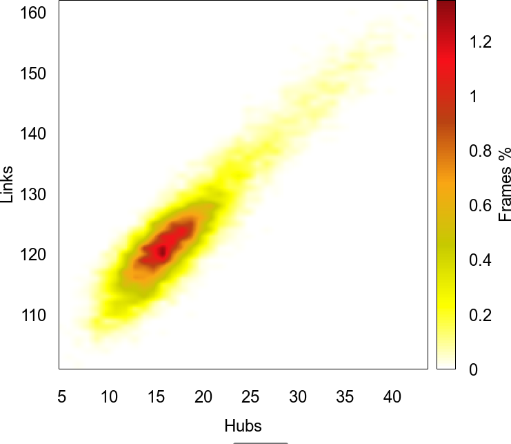
This option is used to add a new distribution or surface plot. At least one plot must be added. When you click on this menu a small window will be opened through which you can choose the type of plot to generate. If Distribution is selected a new window with a list of possible statistics will be shown through which you can choose the distribution to plot. Similarly, if Surface is selected, a window will allow you to choose a pair of statistics to generate a surface plot. This is a composite image of the windows that will be opened after Add Plot → Distribution and Add Plot → Surface:
|

For a detailed list of available network statistics see the corresponding table in Miscellaneous → PSN Info section.
For each distribution and surface plots the following output files will be produced:
| Output | Description |
|---|---|
Dist.: {Stat} Info |
This is a table with some information about the distribution of the network statistic:
|
Dist.: {Stat} Data |
A data file with the values used to generated the corresponding plot mentioned below. |
Surf.: {StatsPair} Info |
This is a table with some information about three most recurrent pairs of values of the two passed statistics:
|
Surf.: {StatsPair} Data |
A text file with the data used to generated the surface plot mentioned below. |
Where {Stat} and {StatsPair} are the network statistic and the pair of network statistics selected while adding the distribution and the surface plots, respectively.
| Output | Description |
|---|---|
{Stat} Dist. |
A plot of the distribution of the statistic values versus the % of trajectory frames. |
{StatsPair} Surf. |
A 2D plot of the joint probability distribution of the statistics values versus the % of trajectory frames. |
Where {Stat} and {StatsPair} are the network statistic and the pair of network statistics selected while adding the distribution and the surface plots, respectively.
Finally, you can close this window using Exit menu.
Plots Of Difference In Trajectory Network Statistics
This analysis is similar to Plots Of Trajectory Network Statistics and is used to calculate the difference in the trajectory network statistics of two different .psn files. To start this analysis click on Analyses → Trajectory Difference Plots menu. The only difference in the setting stage is that you have to provide two psn files. Please refer to Plots Of Trajectory Network Statistics section for more details about the setting and calculation stages.
After the calculation stage, in the Outputs menu, the following outputs will be available:
For each distribution and surface plots the following output files will be produced:
| Output | Description |
|---|---|
Dist.: {Stat} Info |
This is a table with some information about the distribution of the network statistic:
|
Dist.: {Stat} Data |
A data file with the values used to generated the corresponding plot mentioned below. |
Net1 Surf.: {StatsPair} Info |
These files contain some information about three most recurrent pairs of values of the two passed statistics in both networks.
|
Diff. Surf.: {StatsPair} Data |
The data used to generate the 2D plot of the difference of the two joint probability distributions the statistics values versus the % of trajectory frames. |
Net1 Surf.: {StatsPair} Data |
A pair of text files with the data used to generated the plot mentioned above and referring to the first and second .psn file, respectively. |
Where {Stat} and {StatsPair} are the network statistic and the pair of network statistics selected while adding the distribution and the surface plots, respectively.
| Output | Description |
|---|---|
{Stat} Dist. |
A plot of the distributions of the statistic values versus the % of trajectory frames. |
{StatsPair} Surf. |
A pair of 2D plots of the joint probability distribution the statistics values versus the % of trajectory frames in the two passed networks. |
{StatsPair} Diff. Surf. |
A 2D plot of the difference of the two joint probability distributions the statistics values versus the % of trajectory frames. |
Where {Stat} and {StatsPair} are the network statistic and the pair of network statistics selected while adding the distribution and the surface plots, respectively.
Finally, you can close this window using Exit menu.
Labels Menu
Labels files are fundamental when calculating network differences or consensus networks with systems with different primary sequences, with one or more point mutations or simply if their pdb files have different chain and or segments. Despite being a simple two columns file format, compiling a labels file by hand can be a time consuming and error prone task, specially if you have large systems and multiple networks to label.
There are three different ways to automatically generate labels files:
Generate Labels
With this method, labels files are generated from a labels definition file generated by the user. Click on Labels → Generate Labels and enter a new file name when prompted. A new window of selected text editor will be opened with a detailed description of the file format and an example. When finished, close the text editor window and PSNToolsGUI will generate the corresponding labels file for you.
The following table summarize the labels definition file format:
| Column | Description |
|---|---|
1st |
a pdb file name present in the same working directory or with a full disk path |
2nd |
the first residue identifier (see Labels files section) |
3rd |
the last residue identifier |
4th |
the label of the residues defined by the previous two columns (first → last) |
5th |
the starting label number |
This is an example labels definition that can be used to label the chain A residues of the 3LNX pdb:
3lnx.pdb   A:A:P1     A:A:S94    Res     1
3lnx.pdb   A:A:?97    A:A:?102   IOD     1
3lnx.pdb   A:A:?103   A:A:?103   SCN     1
3lnx.pdb   A:A:?104   A:A:?574   Water   1
MSA to Labels
This function is accessible via Labels → MSA To Labels menu and provides an alternative way to produce multiple labels files at the same time from a multi sequence alignment (MSA) in fasta format. All you have to do is select the desired multi sequence alignment file when prompted to.
As for the previous method, PSNToolsGUI needs to access to a pdb file corresponding to the each sequence listed in the msa file. To match sequences and the corresponding pdb files, please change the sequence definition line, i.e. the line after ">" character, with the full disk path of the corresponding pdb file as in the following example:
>3lnx.pdb
PKPGDIFEVELAKNDNSLGISVTGGVNTSVRHGGIYVKAVIPQGAAESDGRIHKGDRVLA
VNGVSLEGATHKQAVETLRNTGQVVHLLLEKGQS

>3lny.pdb
PKEQVSAVVELAKNDNSLGISVTGGVNTSVRHGGIYVKAVIPQGAAESDGRIHKGDRVLA
VNGVSLEGATHKQAVETLRNTGQVVHLLLEKGQS
WebPSN Labels Generator
The easiest way to generate a labels file is to use the corresponding tool provided by WebPSN, the web server version of PSNToolsGUI.
Miscellaneous Menu
In this menu you will find a series of small but helpful additional functions.
Check PDB Parameters
PSNToolsGUI uses the residue type field (4th column) of passed pdb file to assign the correct network parameter to each node during PSN calculation. These three-letters codes are (almost) standardized, nonetheless some molecular simulation programs, like CHARMM or Gromacs, use some codes with an alternative meanings, like HSD, HSE and HSP to identify different protonation state for the histidines. It is a good practice, before a Network Calculation, to check for non standard aminoacids/nucleotides present in your pdb file and to see to which molecule and network parameter they are associated to in the internal database.
To access this function click on Miscellaneous → Check PDB Parameters menu and select a pdb file when prompted.
This command will show you a table with each non standard aminoacids/nucleotides present in passed pdb and their associated molecule name and formula, as well as, their network parameter. If a molecule is not present in the internal database, it will be parametrized on the fly on the basis of its atomic coordinates.
This is the message that this function will show you when the chain A of PDB Code 1U19 is passed:

Change PSN Name
As seen in the previous Analyses sections, if you do not set the network name option, all output files will be named according to the internal network name of passed psn file. If you want to change the internal network name of a psn file, this little function can modify it for you, all you have to do is to select the desired psn file and set a new name when prompted.
PSN Info
This function shows several information listed in the table below about passed .psn file.
| Column | Description |
|---|---|
Date |
Creation date and time of passed .psn file. |
Name |
network name. |
Type |
CNS for consensus network, PSN for all other networks. |
Mol |
Name of the .pdb file name. |
Trj |
Name of the .dcd/.xtc file name. |
NFr |
Number of trajectory frames or 1 if the network was generated from a single .pdb file. |
Sele |
The selection passed to -sele option during network calculation. |
Lab |
The name of labels file passed to -labfile option during network calculation. |
Imin |
Network Imin value (see the relevant theory section for more details). |
Nodes |
The total number of nodes. |
Nets |
If passed .psn file is a consensus network, the total number of networks used to is reported, 1 otherwise. |
PDBs |
The list of .pdb files. |
Corrs |
The total number of node correlations of the atomic fluctuations. |
EmbeddedPDBs |
The total number and the list of embedded coordinates. Please note that listed names may not correspond to those of the original .pdb files. |
TrjStats Sampling |
The value passed to the -trjstatsampling option during network calculation. |
TrjStats |
The total number and the list of saved trajectory statistics. During network calculation the following 24 network descriptors are also computed for each trajectory frame:
Additionally, for each non standard aminoacid/nucleotide present in passed .pdb /trajectory file, the following 10 network descriptors are also computed:
|
Help Menu
Help (PDF)
Open the PDF version of this user guide in your browser (needs a working internet connection).
Help (WEB)
Open the web version of this user guide in your browser (needs a working internet connection).
Version
Show a message with the current version of installed PSNTools and PSNToolsGUI.
Check Update
Checks if a new version of PSNTools and PSNToolsGUI are available (needs a working internet connection).
About
Shows the about window.
Example Networks and Image Gallery
In this section you will a small gallery of the outputs produced with PSNToolsGUI. If you want to play with PSNToolsGUI without the burden of the calculation step, you can download two pre-calculated networks from the WebPSN website:

Appendix A: A Brief Introduction to Protein Structure Network Theory
PSN Calculation
PSN analysis is a product of graph theory applied to protein and nucleic acid structures. A graph is defined by a set of vertices (nodes) and connections (edges) between them. In a PSN, each amino acid residue is represented as a node and these nodes are connected by edges based on the strength of non-covalent interactions between residues. The strength of interaction between residues i and j (Iij) is evaluated as a percentage given by the following equation:
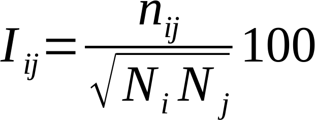
where nij is the number of atom-atom pairs between the side chains of residues i and j within a distance cutoff of 4.5 Å. Ni and Nj are normalization factors for residue types i and j, which account for the differences in size of the amino acid side chains and their propensity to make the maximum number of contacts with other amino acids in protein structures. Glycines, are now included in the PSN analysis. The PSNTools has an internal database with the normalization factors for the 20 standard amino acids and the 8 standard nucleotides (i.e. dA, dG, dC, dT, A, G, C, and U), as well as for more than 30,000 biologically relevant molecules and ions (ligands, lipids, sugars, etc) from the PDB. Additionally, the server automatically identifies un-parametrized molecules in passed PDB files and automatically calculates their normalization factors transparently.
Iij are calculated for all node pairs. At a given interaction strength cutoff, Imin, any residue pair ij for which Iij ≥ Imin is considered to be interacting and hence is connected. Node interconnectivity is used to highlight node clusters, where a cluster is a set of connected nodes in a graph. Cluster size, i.e., the number of nodes constituting a cluster, varies as a function of the Imin, and the size of the largest cluster is used to calculate the Icritic value. The latter is defined as the Imin, at which the size of the largest cluster is half the size of the largest cluster at Imin = 0.0%. Studies by Vishveshwara’s [16] group found that optimal Imin corresponds to the one at which the largest cluster undergoes a transition. All resulting clusters can then be iteratively connected by the link(s) with the highest sub-Icritic interaction strength to compensate, at least in part, for the lack of side chain fluctuations.
Residues making four or more edges are referred to as hubs at that particular Imin. Such cutoff for hub definition relates to the intrinsic limit in the possible number of non covalent connections made by an amino acid in protein structures due to steric constraints. The cutoff 4 is close to the upper limit. The majority of amino acid hubs indeed make from 4 to 6 links, with 4 being the most frequent value. Finally, links are then used to highlight network communities, which are sets of highly interconnected nodes such that nodes belonging to the same community are densely linked to each other and poorly connected to nodes outside the community. Communities can be considered as fairly independent compartments of a graph. They are identified using a variant of the clique percolation method, by finding all the k=3-cliques, i.e. sets of three fully interconnected nodes, and then merging all those cliques sharing at least one node.
Shortest Paths
The search for all shortest paths relies on Dijkstra’s algorithm. The method first finds all possible communication paths between all node pairs and then filters the results according to cross-correlation of atomic motions, as derived from ENM-NMA or LMI analysis for networks calculated from a single .pdb file or from a molecular dynamics simulation, respectively.
Filtering consists in retaining only those shortest paths that contain only residues with a correlation ≥ of a given cutoff with at least one of the two path extremities (i.e. the first and last amino acids in the path). The default values for these cutoffs are 0.7 and 0.8 for networks calculated from a single .pdb file or from a molecular dynamics simulation, respectively and are based on benchmarks tested against experimental data.
Finally, filtered paths were used to build the global meta path, which is made of the most recurrent links, i.e. those links present in a number paths ≥ 10% or 20% for networks calculated from a single .pdb file or from a molecular dynamics simulation, respectively of the number of paths in which the most recurrent link in present. Such meta path represents a coarse/global picture of the structural communication in the considered system. The user can also filter those paths that begin and end at a given residue pair or that pass through a residue. Such a path filtering provides a novel metapath and is particularly recommended when some information on residues involved in structural communication is available.
Appendix B: Correlations of the Atomic Fluctuations
The calculation of the atomic fluctuations is a foundamental step in shortest paths analysis and is automatically performed by PSNTools by means of the latest realease of our Wordom software [18]. Two different kind of
Elastic Network Model Correlations
The combination between a coarse grained representation of a protein structure (e.g. ENM) and Normal Mode Analysis (NMA) is ever increasingly used to study the collective dynamics of complex systems. ENM-NMA is a coarse grained normal mode analysis technique able to describe the vibrational dynamics of protein systems around an energy minimum. With this technique, each protein/nucleic acid structure is described by a reduced subset of atoms corresponding to the Cα atoms, for standard amino acids, and the atom nearest to the geometric center for all other molecules.
The interactions between particle pairs are given by a single term Hookean harmonic potential. The total energy of the system is thus described by the simple Hamiltonian:
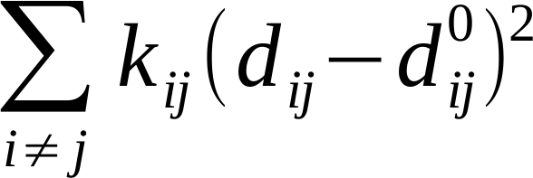
where dij and dij0 are the instantaneous and equilibrium distances between particle i and j, respectively, whereas kij is a force constant, defined as:

where C is constant (with a default value of 40 Kcal/mol ·Å2).
The cross-correlations of motions for path filtering are obtained from the covariance matrix C [17]:
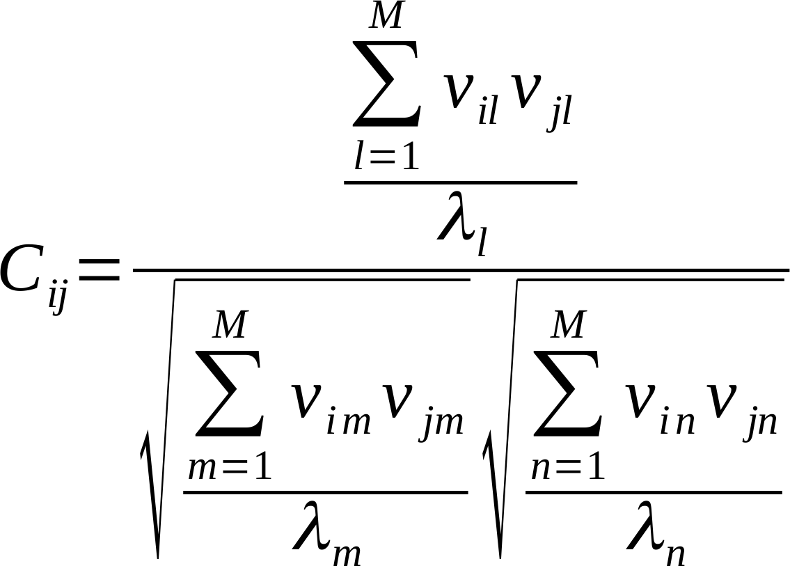
where Cij denotes the correlation between particles i and j, M is the number of modes considered for computation (the first 10 non-zero frequency modes), vxy and λy are, respectively, the xth element and the associated eigenvalue of the yth mode.
Linear Mutual Information Correlations

where i and j ar residues, Cij is the pair-covariance matrix, and Ci and Cj are marginal covariance matrices. LMI correlation values can vary from 0.0 to 1.0, which indicate completely uncorrelated and completely correlated displacements, respectively.
Appendix C: Labels File
When calculating the difference between two networks or a consensus among a pool of networks it is of fundamental importance to unambiguously identify structurally equivalent residues/nucleotides among processed proteins/nucleic acids. A unique identifier, called label, is then associated to these equivalent residues/nucleotides so that their interactions can be compared among the analyzed networks.
There are four possible methods to generate a labels file:
Additionally, you can compile a labels file by hand. Although the compilation of label files may require a considerable amount of time depending on the size and number of analyzed structures, label files provide the user with a full control of the labeling process.
The format of a labels file is quite similar to the one used in external values files: a text file with 2 columns per line, one-residue definition and one label separated by at least one space or tab character, as in the following excerpt:
...
C:S:Y10   Tyr10
C:S:V11   Val11
C:S:P12   Pro12
...
Residues are indicated using the following syntax:
Chain:Segment:ResTypeResNumPlease use one-letter codes for standard amino acids (e.g. P for proline, Y for tyrosine, etc) and the following lower case one-letter codes for standard nucleotides:
| Base | Code |
|---|---|
A, DA |
a |
C, DC |
c |
G, DG |
g |
DT |
t |
U |
u |
Use ? character for any other molecule present in your pdb.
...
C:S:?100   Ligand
C:S:?200   Water
C:S:?300   Mg
...
A label can be a combination of any length of upper and lower case letters (A-Z, a-z), digits (0-9) and all other printable symbols (e.g. !, @, % etc) with the only two exceptions of # and - characters.
Appendix D: External Values File
The user can, optionally, provide numerical values to be associated with any number of residues (e.g. conservation scores, mutation effect, etc.). If provided, these values will appear in the output files (columns OutVal/Value). These values are reported for your convenience only and are not used in any way.
The format of an external values file is quite similar to the one used in labels file: a text file with 2 columns per line, one-residue definition and one label separated by at least one space or tab character, as in the following excerpt:
...
C:S:Y10   7
C:S:V11   7
C:S:P12   5
...
Residues are indicated using the following syntax:
Chain:Segment:ResTypeResNumPlease use one-letter codes for standard amino acids (e.g. P for proline, Y for tyrosine, etc) and the following lower case one-letter codes for standard nucleotides:
| Base | Code |
|---|---|
A, DA |
a |
C, DC |
c |
G, DG |
g |
DT |
t |
U |
u |
Use ? character for any other molecule present in your pdb.
...
C:S:?100   5
C:S:?200   0
C:S:?300   1
...
Appendix E: Selection Syntax
PSNTools adopts a modified version of the selection syntax used in Wordom.
This syntax employs a string structured as follows:
/chain/segment/residues| segment is the 12th field in the pdb (3rd after coordinates). It is a 4-character field, which must not be confused with the chain (single-character) field after the residue-type in the pdb (5th field). |
Wild cards such as * (any number of any character), ? (any single character), [abc] (any single character among a, b and c) and [!abc] (any single character except a, b and c) are supported. Ranges can also be defined using - character.
Syntax       Meaning
/*/*/*       all residues in all chains and segments (default selection)
/C/S/*       all residues in chain C and segment S
/C/S/135     only residue 135 from chain C and segment S
/C/S?/*/*    all residues in chain C and segment S1, SB, SC ...
/C/S[AB]/*   all residues in chain C and segment SA, SB
/C/S/1-32    all residues in the range 1-32 from chain C and segment S
Ranges can be concatenated using the | character
/C/S/1-10|15|20-30selects residues from 1 to 10, 15 and from 20 to 30 from chain C and segment S.
Finally, several selections can be concatenated using the ; character
/A/Q/* ; /B/W/1-10|15 ; /G/E/20-30selects all residues from chain A and segment Q, residues from 1 to 10 and 15 from chain B and segment W and residues from 20 to 30 from chain G and segment E
Appendix F: Color Legends
These are the colors associated to the first nine most populous communities and clusters that will be used when -color option is set to comm or cls, respectively:
| Community/Cluster | 1st | 2nd | 3rd | 4th | 5th | 6th | 7th | 8th | 9th |
|---|---|---|---|---|---|---|---|---|---|
Color |
The following colors are used to represent interaction strength, trajectory frequency and metapath recurrence when -color option is set to force, freq, hfreq, rec, respectively:
| Color | I.S. | Frequency | Recurrence |
|---|---|---|---|
0 < i.s. ≤ 1 |
0 < freq ≤ 10 |
0 < rec ≤ 10 |
|
1 < i.s. ≤ 2 |
10 < freq ≤ 20 |
10 < rec ≤ 20 |
|
2 < i.s. ≤ 3 |
20 < freq ≤ 30 |
20 < rec ≤ 30 |
|
3 < i.s. ≤ 4 |
30 < freq ≤ 40 |
30 < rec ≤ 40 |
|
4 < i.s. ≤ 5 |
40 < freq ≤ 50 |
40 < rec ≤ 50 |
|
5 < i.s. ≤ 6 |
50 < freq ≤ 60 |
50 < rec ≤ 60 |
|
6 < i.s. ≤ 7 |
60 < freq ≤ 70 |
60 < rec ≤ 70 |
|
7 < i.s. ≤ 8 |
70 < freq ≤ 80 |
70 < rec ≤ 80 |
|
8 < i.s. ≤ 9 |
80 < freq ≤ 90 |
80 < rec ≤ 90 |
|
9 < i.s. |
90 < freq ≤ 100 |
90 < rec ≤ 100 |
These three colors are used by -psgdiff, -patsdiff and -tsdiffplots commands:
| Present in | 1st network | both networks | 2st network |
|---|---|---|---|
Color |